Robust stability
In [1]:
import numpy
import matplotlib.pyplot as plt
%matplotlib inline
We will build a simple non-diagonal system with a diagonal proportional controller
In [2]:
W_I = 0.1
K_c = 1

def G(s):
    return numpy.matrix([[1/(s + 1), 1/(s+2)],
                         [0, 2/(2*s + 1)]])
def K(s):
    return K_c*numpy.asmatrix(numpy.eye(2))

def M(s):
    """ N_11 from eq 8.32 """
    return -W_I*K(s)*G(s)*(numpy.eye(2) + K(s)*G(s)).I
In [3]:
M(2.0)
Out[3]:
matrix([[-0.025     , -0.01339286],
        [ 0.        , -0.02857143]])
Let’s observe the MV Nyquist diagram of this process
In [4]:
omega = numpy.logspace(-2, 2, 100)
s = 1j*omega
In [5]:
def mvdet(s):
    return numpy.linalg.det(numpy.eye(2) + G(s)*K(s))

fr = numpy.array([mvdet(si) for si in s])
In [6]:
plt.plot(fr.real, fr.imag)
plt.plot(fr.real, -fr.imag)
plt.axhline(0)
plt.axvline(0)
Out[6]:
<matplotlib.lines.Line2D at 0x11a960208>
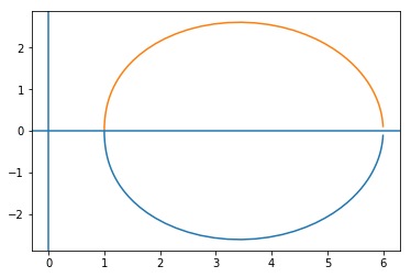
This system looks stable since there are no encirclements of 0.
Now, let’s add some uncertainty. We will be building an unstructured \(\Delta\) as well as a diagonal \(\Delta\).
In [7]:
def maxsigma(m):
    _, S, _ = numpy.linalg.svd(m)
    return S.max()
In [8]:
def specradius(m):
    return numpy.abs(numpy.linalg.eigvals(m)).max()
In [9]:
def unstructuredDelta():
    numbers = numpy.random.rand(4)*2 - 1 + 1j*(numpy.random.rand(4)*2 -1)
    Delta = numpy.asmatrix(numpy.reshape(numbers, (2, 2)))
    return Delta
In [10]:
def diagonalDelta():
    numbers = numpy.random.rand(2)*2 - 1 + 1j*(numpy.random.rand(2)*2 -1)
    Delta = numpy.asmatrix(numpy.diag(numbers))
    return Delta
In [11]:
def allowableDelta(kind):
    while True:
        Delta = kind()
        if maxsigma(Delta) < 1:
            return Delta
So now we can generate an acceptable Delta.
In [12]:
allowableDelta(unstructuredDelta)
Out[12]:
matrix([[ 0.07539216+0.09878427j, -0.73336265+0.2846334j ],
        [-0.51959904+0.5188734j , -0.25490849+0.05011251j]])
In [13]:
I = numpy.eye(2)
In [14]:
def Mdelta(Delta, s):
    return M(s)*Delta
In [15]:
kind = diagonalDelta
Let’s see what the Nyquist diagrams look like for lots of different allowable Deltas.
In [16]:
Ndelta = 200

for i in range(Ndelta):
    Delta = allowableDelta(kind)
    fr = numpy.array([numpy.linalg.det(I - Mdelta(Delta, si)) for si in s])
    plt.plot(fr.real, fr.imag, color='blue', alpha=0.2)
plt.axhline(0, color='black')
plt.axvline(0, color='black')
plt.show()
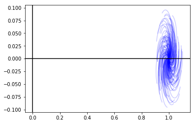
That looks like no \(\Delta\) moved us near the zero point, which is where we will become unstable. So this system looks it’s robustly stable.
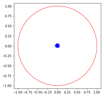
To apply the small gain theorem, we need to check the eigenvalues of \(M\Delta\)
In [17]:
Ndelta = 100
fig = plt.figure(figsize=(5, 5))
for i in range(Ndelta):
    Delta = allowableDelta(kind)
    fr = numpy.array([numpy.linalg.eigvals(Mdelta(Delta, si)) for si in s])
    plt.plot(fr.real, fr.imag, color='blue', alpha=0.2)
plt.gca().add_artist(plt.Circle((0, 0), radius=1, fill=False, color='red'))
plt.axis('equal')
plt.xlim(-1.1, 1.1)
plt.ylim(-1.1, 1.1)
plt.show()
Minimised singular value
How would be find the minimized singular value? One way is via direct optimization.
In [18]:
import scipy.optimize
In [19]:
def obj(d):
    d1, d2 = d
    D = numpy.asmatrix([[d1, 0],
                        [0, d2]])
    return maxsigma(D*M(si)*D.I)
In [20]:
r = scipy.optimize.minimize(obj, [1, 1])
---------------------------------------------------------------------------
NameError                                 Traceback (most recent call last)
<ipython-input-20-77439d733717> in <module>()
----> 1 r = scipy.optimize.minimize(obj, [1, 1])

~/anaconda3/lib/python3.6/site-packages/scipy/optimize/_minimize.py in minimize(fun, x0, args, method, jac, hess, hessp, bounds, constraints, tol, callback, options)
    479         return _minimize_cg(fun, x0, args, jac, callback, **options)
    480     elif meth == 'bfgs':
--> 481         return _minimize_bfgs(fun, x0, args, jac, callback, **options)
    482     elif meth == 'newton-cg':
    483         return _minimize_newtoncg(fun, x0, args, jac, hess, hessp, callback,

~/anaconda3/lib/python3.6/site-packages/scipy/optimize/optimize.py in _minimize_bfgs(fun, x0, args, jac, callback, gtol, norm, eps, maxiter, disp, return_all, **unknown_options)
    941     else:
    942         grad_calls, myfprime = wrap_function(fprime, args)
--> 943     gfk = myfprime(x0)
    944     k = 0
    945     N = len(x0)

~/anaconda3/lib/python3.6/site-packages/scipy/optimize/optimize.py in function_wrapper(*wrapper_args)
    290     def function_wrapper(*wrapper_args):
    291         ncalls[0] += 1
--> 292         return function(*(wrapper_args + args))
    293
    294     return ncalls, function_wrapper

~/anaconda3/lib/python3.6/site-packages/scipy/optimize/optimize.py in approx_fprime(xk, f, epsilon, *args)
    701
    702     """
--> 703     return _approx_fprime_helper(xk, f, epsilon, args=args)
    704
    705

~/anaconda3/lib/python3.6/site-packages/scipy/optimize/optimize.py in _approx_fprime_helper(xk, f, epsilon, args, f0)
    635     """
    636     if f0 is None:
--> 637         f0 = f(*((xk,) + args))
    638     grad = numpy.zeros((len(xk),), float)
    639     ei = numpy.zeros((len(xk),), float)

~/anaconda3/lib/python3.6/site-packages/scipy/optimize/optimize.py in function_wrapper(*wrapper_args)
    290     def function_wrapper(*wrapper_args):
    291         ncalls[0] += 1
--> 292         return function(*(wrapper_args + args))
    293
    294     return ncalls, function_wrapper

<ipython-input-19-97cd97df0c1e> in obj(d)
      3     D = numpy.asmatrix([[d1, 0],
      4                         [0, d2]])
----> 5     return maxsigma(D*M(si)*D.I)

NameError: name 'si' is not defined
In [ ]:
b = []
for si in s:
    r = scipy.optimize.minimize(obj, [4, 4])
    f = r.fun
    b.append(f)
Let’s plot all the spectral radii along with some bounds. Remember you
can go back and change kind to do this for the other kind of ∆.
In [ ]:
Ndelta = 1000

for i in range(Ndelta):
    Delta = allowableDelta(kind)
    specradiuss = numpy.array([specradius(Mdelta(Delta, si)) for si in s])
    plt.loglog(omega, specradiuss, color='blue', alpha=0.2)

maxsigmas = numpy.array([maxsigma(M(si)) for si in s])
specradius_of_m = [specradius(M(si)) for si in s]
plt.loglog(omega, maxsigmas, color='red', label=r'$\bar{\sigma}(M)$')
plt.loglog(omega, specradius_of_m, linewidth=6, color='green', label=r'$\rho{M}$')
plt.loglog(omega, b, linewidth=2, color='yellow', label=r'$\min_D \bar{\sigma}(DMD^{-1})$')
plt.axhline(1, color='black')
plt.ylim([1e-2, 1e-1])
plt.legend()
plt.show()